The new AequilibraE 1.0.1 release brings some major improvements to the graph compression which provide large runtime and memory improvements to all assignment related processes. Assigning our “all of Australia” model runs 13% faster!!! The best part - as these are all under the hood improvements, users don’t have to do anything other than upgrade to get the benefits. To really understand what’s changed though, we have to dig into dead ends and fish spines.

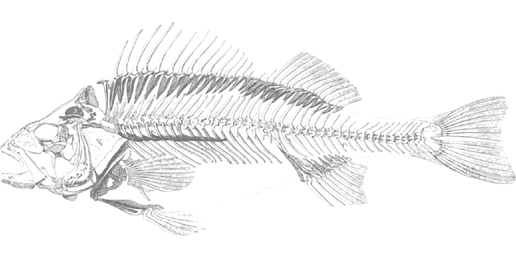
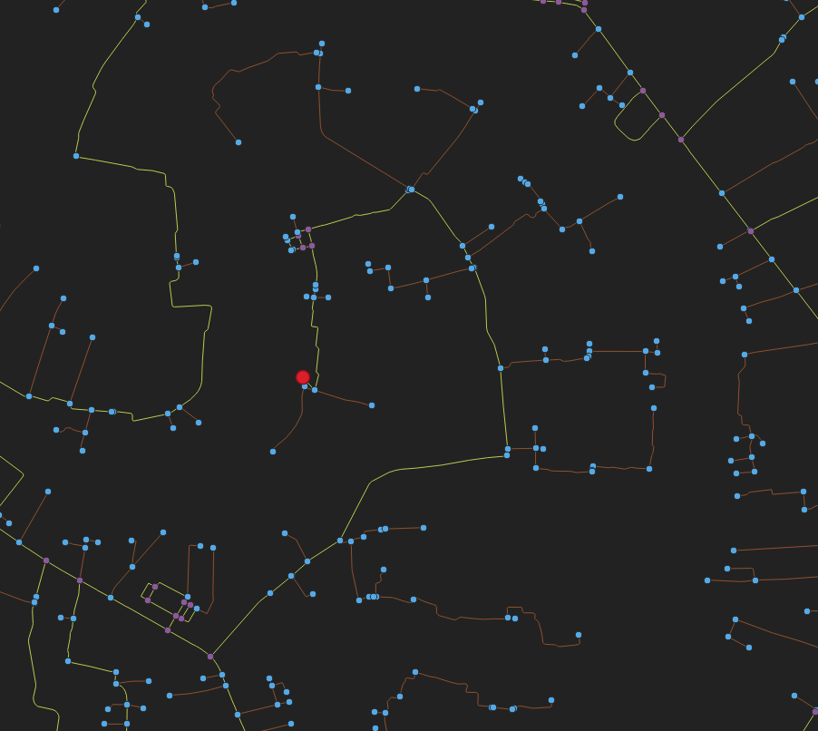
A fish spine, despite its name, is unrelated to aquatic life. Instead, it refers to a specific pattern within high-resolution road networks where a road has multiple smaller streets branching off from it. These branches often lead to dead ends or cul-de-sacs, creating a pattern that, from above, might resemble the spine of a fish. This is particularly notable in suburban and exurban areas. While this detail is important and useful, dead ends are well… dead ends, and while to a human it’s easy to ignore them entirely when planning a route it’s not as easy for computers. Given these fish spines can make up a non-negligible portion of a network it would be useful if a computer could ignore them just as we might.

To justify their exclusion, we rely on the presence of known centroids as the sole origin and destination nodes, coupled with the constraints of time and Euclidean space. This ensures that omitting fish spines won’t compromise our network’s integrity.

As we know all possible origins and destinations, we know we will end (or begin) in a dead end only if that dead end is a centroid. If a dead end is a centroid, then we can simply keep it.

We also know that the cost of a direct path (a -> b) is always less than or equal to a path with detours (a -> c -> d -> b). As all graph weights are known to be non-negative, we know we can’t turn down a dead end and somehow exit with a lower odometer or in the past. This means that the removal of fish spines does not affect the shortest paths produced by Dijkstra’s algorithm, and the short paths produced by A* are unchanged or better.

The removal process for an undirected simple graph (no loops or multi-edges) is simple enough. For all v in G(V, E) such that degree(V) = 1, remove the sequence of links connecting v to the rest of the graph, ensuring all other vertices connected to the removed links have a degree of 2, excluding already removed edges. A potential concern with this method is the undefined order for removing individual strings of links forming dead ends within fish spines. Although the formal proof is not presented here, the general principle is that the removal order does not impact the outcome. To illustrate, initially consider just the root node of the fish spine, then sequentially add the leaf nodes with all connected edges and vertices one at a time. You’ll observe that the order that these leaf nodes are added in does not matter, it always results in the same tree structure. The reverse of this process should demonstrate our argument.

A similar approach can be applied to directed graphs. Instead of removing single bidirectional links, we search for a back edge and remove that as well, if present. Given that all weights are non-negative, identifying the transpose of the edge is unnecessary; any back edge will suffice. However, transitioning to directed graphs introduces a complication: dead ends connected only by incoming edges cannot be eliminated through this process. Theoretically, the solution is straightforward—execute the dead-end removal, transpose the graph, rerun the removal, and then either transpose back or map the removed edges to the original graph. This necessitates constructing a transposed graph for what is considered a rare occurrence thus we don’t remove this case.

To further generalise, we introduce the concept of “no choice” removal. This involves initiating a Breadth First Search (BFS) when all edges are outgoing (or incoming), with no incoming (or outgoing) edges present. Additionally, removal continues when all outgoing (or incoming) edges lead to the same node. This concept is based on the premise that if a pathfinding algorithm were to evaluate a node, it would either have no alternative for its next node or find that the node is inaccessible from any other.

As for performance, this relatively simple process provides some modest improvements. On an Australia-wide model with 2288 centroids (2016 SA2s), the uncompressed mixed graph has 3,552,750 links and 2,666,034 nodes, the uncompressed directed graph blows up to 6,640,976 links. Without the dead-end removal, the existing graph compression is able to knock that down to 3,074,376 links. Skimming this network takes on average ~40s. With the dead-end removal it’s able to knock that down a further ~200k to 2,796,255 links. While that may not seem like too much the dead-end removal is removing 1,810,209 directed links before the existing compression kicks in. This improves the skimming time by ~6s. That’s a ~13% improvement, which is in line with what we would expect the 9% link reduction to produce. All times were produced on a 32c Threadripper 3970X.

The dead-end removal also has an interesting interaction with the existing compression; as the existing compression has to stop when there is a fork in a link sequence, dead end removal can actually turns what was previously an incompressible sequence into a compressible one by reducing the degree of the intermediate nodes to 2.